This instructional is the root of laptop imaginative and prescient delivered as “Lesson 2” of the sequence; there are extra courses upcoming that can communicate to the level of establishing your individual deep learning-based laptop imaginative and prescient initiatives. You’ll be able to to find the whole syllabus and desk of contents right here.
The primary takeaways from this text:
- Loading an Symbol from Disk.
- Acquiring the ‘Peak,’ ‘Width,’ and ‘Intensity’ of the Symbol.
- Discovering R, G, and B elements of the Symbol.
- Drawing the usage of OpenCV.
Loading an Symbol From Disk
Ahead of we carry out any operations or manipulations of a picture, it is vital for us to load a picture of our option to the disk. We can carry out this job the usage of OpenCV. There are two tactics we will carry out this loading operation. A technique is to load the picture through merely passing the picture trail and picture record to the OpenCV’s “imread” serve as. The wrong way is to go the picture via a command line argument the usage of python module argparse.
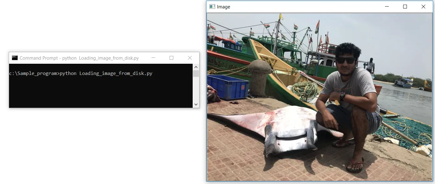
#Loading Symbol from disk

import cv2
picture = cv2.imread(“C:/Sample_program/instance.jpg”)
cv2.imshow(‘Symbol’, picture)
cv2.waitKey(0)
Let’s create a record identify Loading_image_from_disk.py in a notepad++. First, we import our OpenCV library, which comprises our image-processing purposes. We import the library the usage of the primary line of code as cv2. The second one line of code is the place we learn our picture the usage of the cv2.imread serve as in OpenCV, and we go at the trail of the picture as a parameter; the trail will have to additionally include the record identify with its picture layout extension .jpg, .jpeg, .png, or .tiff.
syntax — // picture=cv2.imread(“trail/to/your/picture.jpg”) //
Absolute care needs to be taken whilst specifying the record extension identify. We’re prone to obtain the under error if we give you the mistaken extension identify.
ERROR :

c:Sample_program>python Loading_image_from_disk.py
Traceback (most up-to-date name ultimate):
Record “Loading_image_from_disk.py”, line 4, in <module>
cv2.imshow(‘Symbol’, picture)
cv2.error: OpenCV(4.3.0) C:projectsopencv-pythonopencvmoduleshighguisrcwindow.cpp:376: error: (-215:Statement failed) dimension.width>0 && dimension.peak>0 in serve as ‘cv::imshow’
The 3rd line of code is the place we in truth show our picture loaded. The primary parameter is a string, or the “identify” of our window. The second one parameter is the article to which the picture was once loaded.
In spite of everything, a decision to cv2.waitKey pauses the execution of the script till we press a key on our keyboard. The use of a parameter of “0” signifies that any keypress will un-pause the execution. Please be at liberty to run your program with no need the ultimate line of code to your program to look the variation.
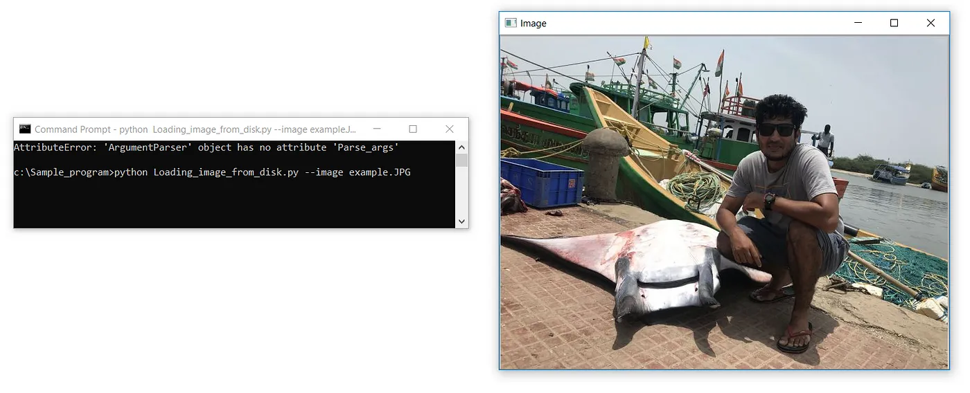
#Studying Symbol from disk the usage of Argparse

import cv2
import argparse

apr = argparse.ArgumentParser()
apr.add_argument(“-i”, “ — picture”, required=True, lend a hand=”Trail to the picture”)
args = vars(apr.parse_args())

picture = cv2.imread(args[“image”])
cv2.imshow(‘Symbol’, picture)
cv2.waitKey(0)
Figuring out to learn a picture or record the usage of a command line argument (argparse) is a fully vital talent.
The primary two strains of code are to import vital libraries; right here, we import OpenCV and Argparse. We can be repeating this right through the route.
The next 3 strains of code maintain parsing the command line arguments. The one argument we want is — picture: the trail to our picture on disk. In spite of everything, we parse the arguments and retailer them in a dictionary referred to as args.
Let’s take a 2nd and briefly speak about precisely what the — picture transfer is. The — picture “transfer” (“transfer” is a synonym for “command line argument” and the phrases can be utilized interchangeably) is a string that we specify on the command line. This transfer tells our Loading_image_from_disk.py script, the place the picture we wish to load lives on disk.
The ultimate 3 strains of code are mentioned previous; the cv2.imread serve as takes args[“image’] as a parameter, which is not anything however the picture we offer within the command recommended. cv2.imshow presentations the picture, which is already saved in a picture object from the former line. The ultimate line pauses the execution of the script till we press a key on our keyboard.
Probably the most primary benefits of the usage of an argparse — command line argument is that we can load photographs from other folder places with no need to modify the picture trail in our program through dynamically passing the picture trail Ex — “ C:CV_Materialimagesample.jpg “ within the command recommended as a controversy whilst we execute our python program.

c:Sample_program>python Loading_image_from_disk.py — picture C:CV_Materialsession1.JPG
Right here, we’re executing the Loading_image_from_disk.py python record from c:sample_program location through passing the “-image” parameter along side the trail of picture C:CV_Materialsession1.JPG.
Acquiring the ‘Peak’, ‘Width’ and ‘Intensity’ of Symbol
Since photographs are represented as NumPy arrays, we will merely use the .form characteristic to inspect the width, peak, and selection of channels.
By way of the usage of the .form characteristic at the picture object we simply loaded. We will to find the peak, Width, and Intensity of the picture. As mentioned within the earlier lesson — 1, the Peak and width of the picture will also be cross-verified through opening the picture in MS Paint. Consult with the former lesson. We can speak about in regards to the intensity of picture within the upcoming courses. Intensity is often referred to as channel of a picture. Coloured photographs are in most cases of three channel on account of the RGB composition in its pixels and gray scaled photographs are of one channel. That is one thing we had mentioned within the earlier Lesson-1.
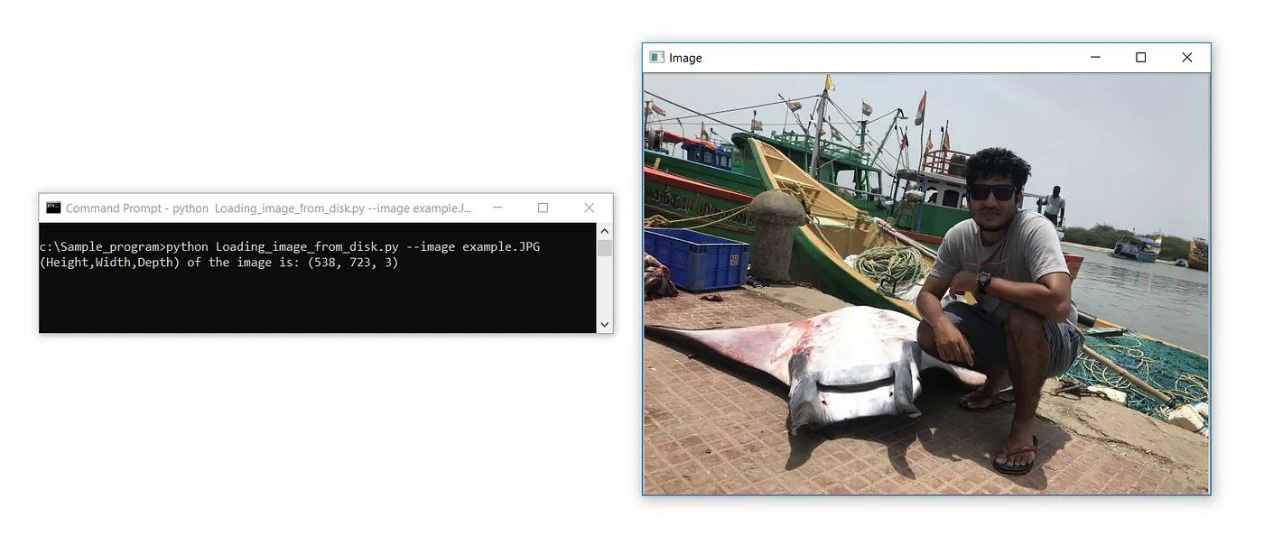
#Acquiring Peak,Width and Intensity of an Symbol

import cv2
import argparse

apr = argparse.ArgumentParser()
apr.add_argument(“-i”, “ — picture”, required=True, lend a hand=”Trail to the picture”)
args = vars(apr.parse_args())

# Simplest distinction to the former codes — form characteristic implemented on picture object

print(f’(Peak,Width,Intensity) of the picture is: {picture.form}’)

picture = cv2.imread(args[“image”])
cv2.imshow(‘Symbol’, picture)
cv2.waitKey(0)
Output:
(Peak, Width, Intensity) of the picture is: (538, 723, 3)
The one distinction from the former codes is the print remark that applies the form characteristic to the loaded picture object. f’ is the F-string @ formatted string that takes variables dynamically and prints.
f’ write anything else right here that you wish to have to look within the print remark: {variables, variables, object, object.characteristic,}’
Right here, we have now used {object.characteristic} within the flower bracket for the .form characteristic to compute the picture object’s peak, width, and intensity.
#Acquiring Peak,Width and Intensity one by one

import cv2
import argparse

apr = argparse.ArgumentParser()
apr.add_argument(“-i”, “ — picture”, required=True, lend a hand=”Trail to the picture”)
args = vars(apr.parse_args())

picture = cv2.imread(args[“image”])

# NumPy array chopping to acquire the peak, width and intensity one by one

print(“peak: %d pixels” % (picture.form[0]))
print(“width: %d pixels” % (picture.form[1]))
print(“intensity: %d” % (picture.form[2]))

cv2.imshow(‘Symbol’, picture)
cv2.waitKey(0)Output:
width: 723 pixels
peak: 538 pixels
intensity: 3
Right here, as an alternative of acquiring the (peak, width, and intensity) in combination as a tuple. We carry out array chopping and procure the peak, width, and intensity of the picture for my part. The 0th index of array comprises the peak of the picture, 1st index comprises the picture’s width, and 2d index comprises the intensity of the picture.
Discovering R, G, and B Parts of the Symbol

Output:
The Blue Inexperienced Pink element price of the picture at place (321, 308) is: (238, 242, 253)
Realize how the y price is handed in ahead of the x price — this syntax would possibly really feel counter-intuitive at first, however it’s in step with how we get right of entry to values in a matrix: first we specify the row quantity, then the column quantity. From there, we’re given a tuple representing the picture’s Blue, Inexperienced, and Pink elements.
We will additionally trade the colour of a pixel at a given place through reversing the operation.
#Discovering R,B,G of the Symbol at (x,y) place

import cv2
import argparse

apr = argparse.ArgumentParser()
apr.add_argument(“-i”, “ — picture”, required=True, lend a hand=”Trail to the picture”)
args = vars(apr.parse_args())

picture = cv2.imread(args[“image”])

# Obtain the pixel co-ordinate price as [y,x] from the person, for which the RGB values needs to be computed
[y,x] = listing(int(x.strip()) for x in enter().cut up(‘,’))

# Extract the (Blue,inexperienced,purple) values of the gained pixel co-ordinate
(b,g,r) = picture[y,x]
print(f’The Blue Inexperienced Pink element price of the picture at place {(y,x)} is: {(b,g,r)}’)

cv2.imshow(‘Symbol’, picture)
cv2.waitKey(0)
(b,g,r) = picture[y,x] to picture[y,x] = (b,g,r)
Right here we assign the colour in (BGR) to the picture pixel co-ordinate. Let’s take a look at through assigning RED colour to the pixel at place (321,308) and validate the similar through printing the pixel BGR on the given place.
#Reversing the Operation to assign RGB price to the pixel of our selection

import cv2
import argparse

apr = argparse.ArgumentParser()
apr.add_argument(“-i”, “ — picture”, required=True, lend a hand=”Trail to the picture”)
args = vars(apr.parse_args())

picture = cv2.imread(args[“image”])

# Obtain the pixel co-ordinate price as [y,x] from the person, for which the RGB values needs to be computed
[y,x] = listing(int(x.strip()) for x in enter().cut up(‘,’))

# Extract the (Blue,inexperienced,purple) values of the gained pixel co-ordinate
picture[y,x] = (0,0,255)
(b,g,r) = picture[y,x]
print(f’The Blue Inexperienced Pink element price of the picture at place {(y,x)} is: {(b,g,r)}’)

cv2.imshow(‘Symbol’, picture)
cv2.waitKey(0)
Output:
The Blue, Inexperienced, and Pink element values of the picture at place (321, 308) are (0, 0, 255)
Within the above code, we obtain the pixel co-ordinate throughout the command recommended through getting into the price as proven within the under Fig 2.6 and assign the pixel co-ordinate purple colour through assigning (0,0,255) ie,(Blue, Inexperienced, Pink) and validate the similar through printing the enter pixel co-ordinate.
Drawing The use of OpenCV
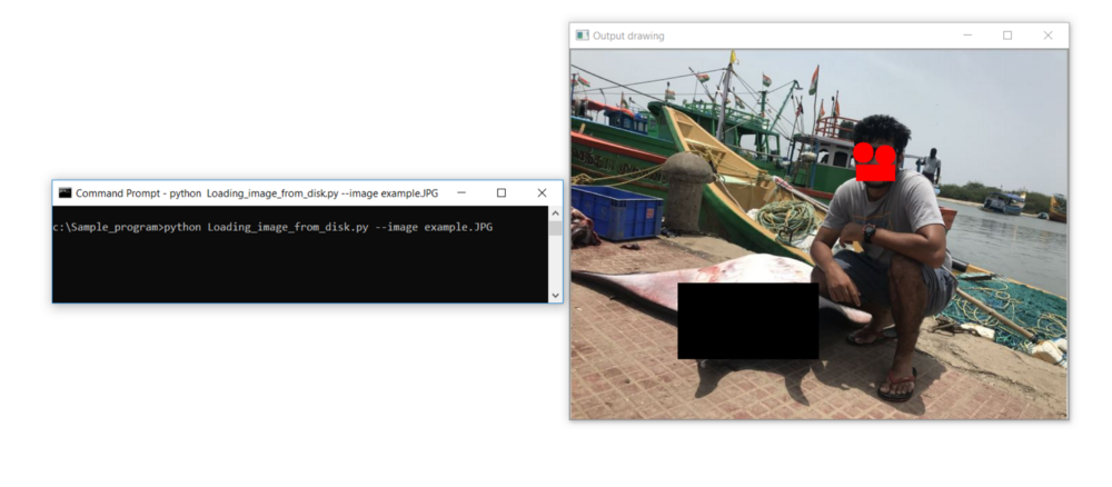
Let’s learn to draw other shapes like rectangles, squares, and circles the usage of OpenCV through drawing circles to masks my eyes, rectangles to masks my lips, and rectangles to masks the mantra-ray fish subsequent to me.
The output will have to seem like this:
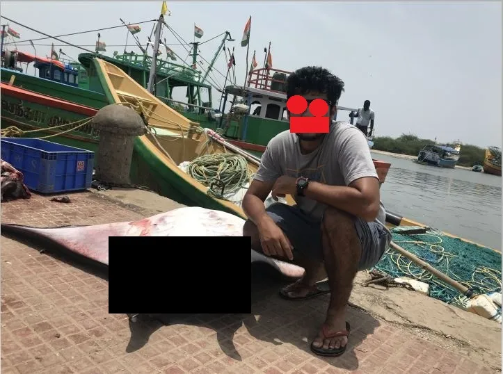
This picture is masked with shapes the usage of MS Paint; we will be able to attempt to do the similar the usage of OpenCV through drawing circles round my eyes and rectangles to masks my lips and the matra-ray fish subsequent to me.
We use cv2.rectangle way to attract a rectangle and cv2.circle way to attract a circle in OpenCV.
cv2.rectangle(picture, (x1, y1), (x2, y2), (Blue, Inexperienced, Pink), Thickness)
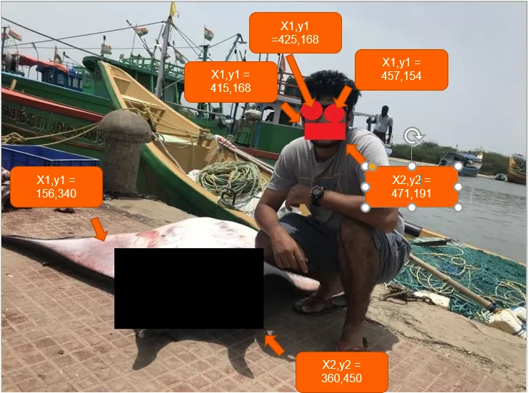
The cv2.rectangle way takes a picture as its first argument on which we wish to draw our rectangle. We wish to draw at the loaded picture object, so we go it into the process. The second one argument is the beginning (x1, y1) place of our rectangle — right here, we’re beginning our rectangle at issues (156 and 340). Then, we should supply an finishing (x2, y2) level for the rectangle. We make a decision to finish our rectangle at (360, 450). The next argument is the colour of the rectangle we wish to draw; right here, on this case, we’re passing black colour in BGR layout, i.e.,(0,0,0). In spite of everything, the ultimate argument we go is the thickness of the road. We give -1 to attract forged shapes, as observed in Fig 2.6.
In a similar way, we use cv2.circle way to attract the circle.
cv2.circle(picture, (x, y), r, (Blue, Inexperienced, Pink), Thickness)
The cv2.circle way takes a picture as its first argument on which we wish to draw our rectangle. We wish to draw at the picture object that we have got loaded, so we go it into the process. The second one argument is the middle (x, y) place of our circle — right here, we have now taken our circle at level (343, 243). The next argument is the radius of the circle we wish to draw. The next argument is the colour of the circle; right here, on this case, we’re passing RED colour in BGR layout, i.e.,(0,0,255). In spite of everything, the ultimate argument we go is the thickness of the road. We give -1 to attract forged shapes, as observed in Fig 2.6.
Good enough ! By way of realizing all this. Let’s attempt to accomplish what we began. To attract the shapes within the picture, we wish to determine the covering area’s beginning and finishing (x,y) coordinates to go it to the respective way.
How?
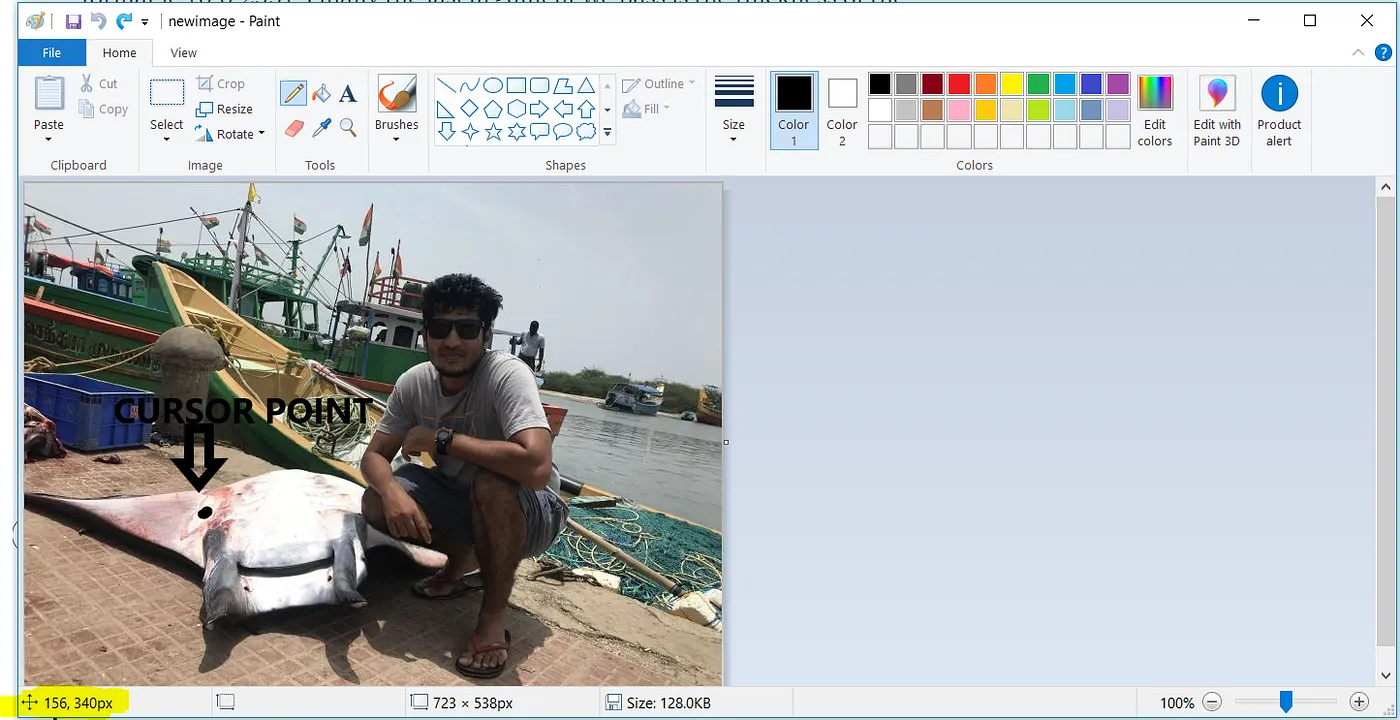
We can take the assistance of MS Paint for another time. By way of striking the cursor over some of the co-ordinate (best left) or (backside proper) of the area to masks, the co-ordinates are proven within the highlighted portion of the MS Paint as proven in Fig 2.7.
In a similar way we will be able to take the entire co-ordinate (x1,y1) (x2,y2) for the entire covering areas as proven within the Fig 2.8.
#Drawing the usage of OpenCV to masks eyes,mouth and object near-by

import cv2
import argparse

apr = argparse.ArgumentParser()
apr.add_argument(“-i”, “ — picture”, required=True, lend a hand=”Trail to the picture”)
args = vars(apr.parse_args())

picture = cv2.imread(args[“image”])

cv2.rectangle(picture, (415, 168), (471, 191), (0, 0, 255), -1)
cv2.circle(picture, (425, 150), 15, (0, 0, 255), -1)
cv2.circle(picture, (457, 154), 15, (0, 0, 255), -1)
cv2.rectangle(picture, (156, 340), (360, 450), (0, 0, 0), -1)

# display the output picture
cv2.imshow(“Output drawing “, picture)
cv2.waitKey(0)
Outcome: